Dose Administration
So far we have considered only a bolus dose - a single amount administered instantaneously to a given compartment, either intravenously (e.g. an injection) or via absorption (e.g. an orally administered pill).
There are, of course, other means of administering a drug and here we will introduce the dosing functions supported by PoPy. All of the dosing functions have two arguments in common:
- the amt argument is the quantity of drug administered in total.
- the lag argument defines a delay between the drug being administered (as specified in the data file) and the drug entering the compartment where it is administered. This can be useful when very little drug is absorbed immediately. Unless otherwise stated, it is assumed that the lag time is zero.
The remaining arguments to the dosing function are dependent on the dose type.
Bolus Dose
A bolus dose represents an instantaneous increase in the amount of a drug in a specific compartment. Physiologically it represents an injection where the drug is assumed to be well distributed within the compartment within a negligible time period.
Note
See the Bolus Dose with no elimination. for Tut Script used to generate results in this section.
The mathematical expression for a bolus at time  in compartment Central is:-
![s[CENTRAL] = s[CENTRAL] + B(t)](../../_images/math/1a27fd400489e576ca3f59083f94a76697903f16.png)
where:-
![B(t)=
\Biggl \lbrace
{
\text{c[AMT]} ,\text{ if } { t = t_B }
\atop
0.0, \text{ otherwise }
}](../../_images/math/56ee6bd9a1699cb71f2dced0667bf627c7181a07.png)
In PoPy, we add a bolus dose to a given compartment (e.g. Central) using the DERIVATIVES section of the script:
d[CENTRAL] = @bolus{amt: c[AMT], lag: m[LAG]} + ...
Because the dose amount is usually fixed by the experiment, it is typically included in the input data and is therefore a column (or covariate) and encoded as such, e.g. c[AMT].
The lag time, however, is usually estimated as a model parameter and would typically be coded as such, e.g. m[LAG]. If lag time is not included in the bolus function, it defaults to zero:
d[CENTRAL] = @bolus{amt: c[AMT], lag: 0.0} + ...
which is exactly the same as
d[CENTRAL] = @bolus{amt: c[AMT]} + ...
See @bolus for some more syntax examples.
The cumulative amount in the compartment (with no elimination) is therefore a step function (Fig. 21):

Fig. 21 Cumulative amount following a bolus dose with no elimination
An example of a bolus dose added to a one compartment model with no lag time is:
DERIVATIVES: |
    d[CENTRAL] = @bolus{amt:c[AMT]} - c[CL]*s[CENTRAL]/c[V]
Infusion
An infusion administers the dose gradually, usually at a fixed rate over a fixed period of time (i.e. the rate of infusion is constant during the time period and zero before and after, typically intravenously).
The mathematical expression for an infusion is:
![\text{d[CENTRAL]} = \text{d[CENTRAL]} + \text{R(t)}](../../_images/math/e6f6923da3a5a7bdcf53039ffe25b7bc0017b47f.png)
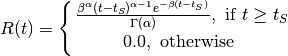
where the infusion has constant rate c[RATE], starts at time t=0 and has duration c[DUR] and in compartment CENTRAL is:-
where:-
![R(t)=
\Biggl \lbrace
{
c[RATE] ,\text{ if } { t_S \leq t \leq t_S + c[DUR] }
\atop
0.0, \text{ otherwise }
}](../../_images/math/cd85af1d4ec138f882d4f757787baa1967900120.png)
An infusion dose can be characterised either by the duration of the infusion or the rate of the infusion.
Note: For a constant total infusion amount (AMT) the RATE and DURATION can be calculated from each other:

So specifying either a RATE or DURATION, together with a total amount, is sufficient to fully define an infusion.
Infusion Duration
An infusion duration is coded by:
@inf_dur{amt: c[AMT], lag: m[LAG], dur: c[DUR]}
in the equation for the appropriate compartment in the DERIVATIVES: section of a fit or tutorial script.
Dose and lag are coded in the same way as for a bolus dose.
Duration can either be included in the input data or can be estimated as a parameter.
Note
See the Infusion Duration Dose with no elimination. for Tut Script used to generate results in this section.
An example of an infusion dose spread over 20 time units added to a one compartment model with no lag time is:
DERIVATIVES: |
    d[CENTRAL] = (
        @inf_dur{amt: c[AMT], lag: 0.0, dur: 20}
        - m[KE]*s[CENTRAL]
    )
If the infusion duration varies between individuals use:
DERIVATIVES: |
    d[CENTRAL] = (
        @inf_dur{amt: c[AMT], lag: 0.0, dur: c[DUR]}
        - m[KE]*s[CENTRAL]
    )
See @inf_dur for some more syntax examples.
The Amount-vs-Time curve for an infusion (without elimination) is a ramp function where the cumulative dose rises linearly until it reaches the total amount administered (Fig. 22).

Fig. 22 Cumulative amount following a infusion dose of 95 mg over a duration of 19 min with no elimination
Infusion Rate
An infusion duration is coded by:
@inf_rate{amt: c[AMT], lag: m[LAG], rate: c[RATE]}
in the equation for the appropriate compartment in the DERIVATIVES: section of a fit or tutorial script.
The amount and lag are coded in the same way as for a bolus dose.
Infusion rate can either be included in the input data or can be estimated as a parameter.
Note
See the Infusion Rate Dose with no elimination. for Tut Script used to generate results in this section.
An example of an infusion dose at a rate of 5 dose units per time unit added to a one compartment model with no lag time is:
DERIVATIVES: |
    d[CENTRAL] = (
        @inf_rate{amt: c[AMT], lag: 0.0, rate: 5}
        - m[KE]*s[CENTRAL]
    )
If the infusion rate is different between individuals use:
DERIVATIVES: |
    d[CENTRAL] = (
        @inf_rate{amt: c[AMT], lag: 0.0, rate: c[RATE]}
        - m[KE]*s[CENTRAL]
    )
See @inf_rate for some more syntax examples.

Fig. 23 Cumulative amount following a infusion dose of 95 mg at a rate of 5 mg/min with no elimination
Gamma Dose
This occurs when the release of the drug into a specific compartment follows a Gamma curve. See:-
https://en.wikipedia.org/wiki/Gamma_distribution
Note
See the Gamma Dose with no elimination. for Tut Script used to generate results in this section.
The mathematical expression for an Gamma dose starting at time  with Weibull parameters
  and
and  and total dose amount
  in compartment Central is:-
where:-
Where R(t) is the rate of drug absorption at time (t) and and are parameters of the Gamma. R(t) is the Gamma density function scaled by the AMT parameter. Since a density function has unit area under the curve, the AMT scaling ensures that the total dose administered is equal to AMT.
This can be implemented in PoPy using:
@gamma{amt: c[AMT], lag: m[LAG], alpha: m[ALPHA], beta: m[BETA]}
in the equation for the appropriate compartment in the DERIVATIVES section of a Fit Script or ref:tut_script. See @gamma.
Here the parameters map to the Gamma equation as follows:-
| Parameter | Symbol |
|---|---|
| alpha |  |
| beta |  |
The lag is coded in the same way as for a bolus dose. A lag time merely delays the start time of the gamma dose.
An example of a gamma dose added to a one compartment model with no lag time is:
DERIVATIVES: |
    d[CENTRAL] = @gamma{amt: c[AMT], alpha: m[ALPHA], beta: m[BETA]} - m[KE]*s[CENTRAL]

Fig. 24 Cumulative amount following a Gamma dose with no elimination
Weibull Dose
The examples given so far have shown the amount of drug absorbed with respect to time, rising from an initial value (typically zero) to the amount administered.
They can, alternatively, be viewed as the cumulative probability of 1 mg of drug having been absorbed at any given time, multiplied by the total amount (in mg) of drug administered. (Because a density function has unit area under the curve, the scaling ensures that the total dose administered is equal to AMT.) This formulation allows us to consider alternative dosing functions by using different probability distributions.
Note
See the Weibull Dose with no elimination. for Tut Script used to generate results in this section.
One choice that has been proposed [Piotrovskii1987] uses the Weibull distribution [Christensen1980] where the amount,  , absorbed at time
  following a dose of AMT at time
  is given by
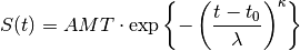
such that
where λ (lambda) and κ (kappa) are, respectively, scale and shape parameters of the Weibull distribution.
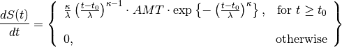
In other words, for 
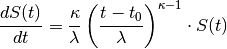
which can be viewed as a rate absorption constant that varies over time, reflecting the possibility that a molecule of drug may be more likely to be absorbed the longer it is resident in the body (for example, due to passage of the drug into the intestine).
A shortcut for the Weibull dosing function is applied in PoPy using
@weibull{amt: c[AMT], lag: m[LAG], lambda: m[LAMBDA], kappa: m[KAPPA]}
in the equation for the appropriate compartment in the DERIVATIVES section of an input script.
The lag works in the same way as for a bolus dose, delaying the onset of the weibull dose. Again, this can be left out if we assume no lag:
DERIVATIVES: |
    d[CENTRAL] = @weibull{amt: c[AMT], lambda: m[LAMBDA], kappa: m[KAPPA]}

Fig. 25 Cumulative amount following a Weibull dose with no elimination
Repeated Dosing
There need not be only one dose administered to the subject for a given experiment – several doses may be given, for example to maintain drug concentration at a steady state over a period of time. PoPy handles this by allowing multiple dose lines in the data file and superimposing the resulting curves, see Table 19.
| Repeated Bolus Dosing | Repeated Infusion Dosing |

|

|
| Repeated Gamma Dosing | Repeated Weibull Dosing |

|

|
Note
See Repeated Bolus Dose with first order elimination., Repeated Infusion Rate Dose with first order elimination., Repeated Gamma Dose with first order elimination. and Repeated Weibull Dose with first order elimination. for the tutorial scripts used to generate results in this section.
Note PoPy can superimpose consecutive complex Dosing Functions (e.g. Weibull and Gamma functions) that can cause numerical instability in other PK/PD packages.