Covariates
Within a population, there will be variability in structural model parameters (such as clearance and volume of distribution) from one individual to another that can be predicted as a function of a measurable property (such as renal function impairment). These measurable properties are known as covariates.
If the variability can be expressed as a deterministic function of these underlying properties, we can model it to increase the accuracy of our predicted time course and decrease the burden on the residual error model.
Continuous Covariates
Continuous covariates appear on a sliding scale that can take on any value (often within a sensible range), as opposed to Discrete Covariates that take one of a finite (and often small) number of values.
We encode the effect of covariate c[Y] on model parameter m[X] via mathematical functions in the MODEL_PARAMS section of the PoPy script. For example, we may assume a linear relationship
m[X] = f[X] + f[X_Y_EFFECT]*c[Y]
though this can permit m[X] to be negative which is undesirable for many model parameters. Alternatives that avoid this problem include the exponential function
m[X] = f[X] * exp(f[X_Y_EFFECT]*c[Y])
or the power function
m[X] = f[X] * c[Y]**f[X_Y_EFFECT]
among others.
It may also be sensible to standardize the covariate in some way, for example by shifting
m[X] = f[X] * (c[Y]-Yref)**f[X_Y_EFFECT]
or scaling
m[X] = f[X] * (c[Y]/Yref)**f[X_Y_EFFECT]
the covariate with respect to some reference value, Yref. Choosing a value that is close to the middle of the range of the data (body weight, for example, is conventionally centred at 70 kg) reduces the correlation between the intercept and the covariate slope, which leads to smaller standard errors and means that the intercept has a sensible interpretation (e.g. CL in an individual with GFR of 120 mL/min).
Body Weight as a Covariate
Note
See Body Weight Covariate for the Tut Script used to generate results in this section.
Empirical studies have shown that the volume of distribution (and clearance, among others) increases with body weight. In the supplied tutorial example, we have added a weight effect coefficient to the fixed effects in the POP level of EFFECTS and a weight covariate at the ID level:
EFFECTS:
    POP: |
        f[KA] = 0.3
        f[CL] = 3
        f[V] = 20
        f[PNOISE] = 0.1
        f[ANOISE] = 0.05
        f[WT_EFFECT] = 0.75  # new fixed effect
    ID: |
        c[ID] = sequential(30)
        c[AMT] = 100.0
        t[RESET] = 0.0
        t[DOSE] = 1.0
        t[OBS] ~ unif(1.0, 50.0; 4)
        c[WT] ~ norm(70, 100)  # new covariate
We then update the MODEL_PARAMS section to include the covariate effect as per the “allometric function” [Holford1996]
MODEL_PARAMS: |
    m[KA] = f[KA]
    m[CL] = f[CL]*(c[WT]/70)**f[WT_EFFECT]  # new covariate effect
    m[V] = f[V]*(c[WT]/70)  # new covariate effect
    m[PNOISE] = f[PNOISE]
    m[ANOISE] = f[ANOISE]
which is a form of power function, using a scaled weight with 70 kg as the reference (as is now accepted in the literature).
This generates a population with time courses that are weight dependent (Fig. 39).

Fig. 39 Simulated prediction curves for a population of 40 individuals with weight-dependent clearance, CL, and volume of distribution, V
For fitting, we estimate only the baseline (median) volume of distribution, f[V], and the weight effect coefficient, f[WT_EFFECT], and we see that the estimated values,
f[KA] = 0.3000
f[CL] = 3.0000
f[V] = 20.2610
f[PNOISE] = 0.1000
f[ANOISE] = 0.0500
f[WT_EFFECT] = 0.6655
closely match those used to generate the observations.
Other Continous Covariates
Other continuous covariates include
- Age: Renal and hepatic functions decrease with age, which can lead to a reduced drug clearance. The volume of distribution of some lipid soluble drugs also increases with age.
- Ideal Body Weight (IBW):
Lean Body Weight (LBW):
Height: The height of an individual, usually measured in cm or m.
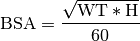
Body Surface Area (BSA): The surface area of the body in m2 can be calculated using the weight in Kg and height in cm. There are various different methods for achieving this such as the Du Bois formula:

or Mosteller formula:
Body Mass Index(BMI): The mass or weight of a subject in kg divided by the square of the height in m, gives the BMI measured in kg/m2

Discrete Covariates
Discrete covariates take one of a finite (and often small) number of values, as opposed to continuous covariates that lie on a spectrum. Discrete covariates can then be used to model differences between groups by allowing a different median value in each group.
Where the covariate represents an either-or classification (i.e. the covariate is dichotomous), we can encode group membership with a zero (reference group) or one (other group). We can then use this indicator variable in a mathematical formula,
m[X] = (1-c[Y])*f[X_WHEN_Y_IS_ZERO] + c[Y]*f[X_WHEN_Y_IS_ONE]
For ease of interpretation, PoPy allows you to encode data columns as strings so that you can see immediately which group is being referred to in the input file. In these cases, an if-else statement can be used to apply the correct fixed effect to the model parameter. This method, unlike indicator variables, can also be used for discrete variables that take more than two values (e.g. race).
if c[Y] == 'zero':
    m[X] = f[X_WHEN_Y_IS_ZERO]
elif c[Y] == 'one':
    m[X] = f[X_WHEN_Y_IS_ONE]
elif c[Y] == 'two':
    m[X] = f[X_WHEN_Y_IS_TWO]
...
We refer to discrete covariates that assign to a group as categorical covariates.
In contrast, ordinal covariates are a discretization of the continuous spectrum and have a definite ordering. These values can sometimes be treated as if they are continuous (e.g. the Child-Pugh scale for hepatic impairment) but it is up to the modeller to decide whether this is justifiable.
Other Discrete Covariates
Other discrete covariates include:
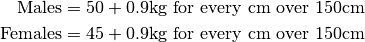
Sex
Females may have different volumes of distribution or clearances (or both) than men for some drugs, even after the difference in body weight is accounted for.
Race
In some cases, race categorizations may be associated with different pharmacokinetic parameters. For example, the frequency of genetic polymorphisms affecting clearance can vary with race.
Concomitant Medication
When two or more drugs are administrated concurrently, they may interfere with each others pharmacokinetic profiles by competing for metabolizing enzymes or transporters. Drugs can also alter the transcription of enzymes, transporters or proteins within drug-binding sites, which can alter both their own pharmacokinetics and the pharmacokinetics of co-administered drugs.
For example, Drug A, or its metabolites, could induce an enzyme for a conjugation reaction in the metabolisation of Drug B. In this case, Drug A could increase the clearance of Drug B.
Alternatively, Drug A, or its metabolites could be an inhibitor on one of the enzymes facilitating the metabolism of Drug B. In this case, Drug A could decrease the clearance of Drug B.
The interactions of different drugs and their metabolites can be very complex and are an important area for population pharmacokinetic modelling.
Smoking
Smoking cigarettes increases the clearance of some drugs by increasing the activity of enzymes used in hepatic metabolism. Caffeine is an example of a drug that has increased clearance in smokers. Note that it is not usually the nicotine in cigarettes that affects metabolism, but other chemicals in the cigarette smoke. Nicotine replacement therapy may not have the same effect.
Disease state
Many diseases or conditions can alter pharmacokinetics. An example is oedema, which causes an excess of fluid in cavities or tissues in the body. If a drug is soluble in this fluid, it could increase the volume of distribution.
Food intake
If a drug is administered orally, the rate of absorption can be affected by whether an individual has eaten recently or not. This is because most drugs are absorbed through the small intestine, but to reach this they have to pass through the stomach. When food is present in the stomach, gastric secretion and residence time are increased. This could lead to a slower absorption rate.