Compartment Models
Although analytic solutions exist for simple models, more complex models can be difficult (or impossible) to define in closed form. Compartment models are a basic tool used to describe more complex PK in animals and man, the idea being that the body can be treated as though it were composed of a number of compartments through which the drug disperses. The concentration of drug in some of these compartments can be measured directly, e.g. by taking blood samples.
A typical model contains a Central compartment that represents the site of sampling (usually the blood plasma) with zero or more additional compartments. Drug diffuses between compartments (sometimes under the action of transporters) as the system heads toward an equilibrium state in which concentrations in each compartment may or may not be equal.
Drug is lost over time from the Central compartment via elimination (usually through the action of the liver and kidneys).
Note
Compartmental models are not intended to replicate biology per se; they simply produce mathematical curves that resemble observations, and it is difficult to associate any compartment with a specific tissue or organ unless sampling occurs at that site.
One Compartment Model
One Compartment Model with Intravenous Dosing
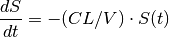
We return to the example from the previous chapter whereby a 100 mg bolus dose of drug is administered intravenously into the body, which we now refer to as the Central compartment. The drug is then removed from the Central compartment by the same process of elimination described previously, such that
which has the closed form solution

Note
See the One Compartment Model with Intravenous Dosing for Tut Script used to generate results in this section.
Graphically, we can draw a compartment diagram that shows the flows into and out of the Central compartment (Fig. 9).

Fig. 9 Compartment diagram for a one compartment model with intravenous dosing.
In the previous chapter, we specified this model programatically by writing the closed form solution directly into the PREDICTIONS block of the control script:
PREDICTIONS: |
    plabel[DRUG_CONC] = "Drug Concentration (mg/L)"
    clabel[TIME] = "Time (minutes)"
    AMOUNT = c[AMT]*exp(-(c[CL]/c[V])*(c[TIME]-1.0))
    p[DRUG_CONC] = AMOUNT/c[V]
    c[DRUG_CONC] ~ norm(p[DRUG_CONC], 0.0)
Using the compartment model approach, however, we can express the same model more naturally using the differential equations themselves, and obtain amounts (and therefore concentrations) using a numerical ODE solver. To do so, we need to add a new section, DERIVATIVES, to the control script in which we specify the differential equations:
DERIVATIVES: |
    d[CENTRAL] = @bolus{amt:c[AMT]} - c[CL]*s[CENTRAL]/c[V]
where d[CENTRAL] represents the first derivative of the amount of drug, s[CENTRAL], in the Central compartment.
There are two components of the flow: a positive flow, representing an intravenous bolus dose, into the Central compartment
@bolus{amt: c[AMT]}
and a negative flow out of the Central compartment,
-c[CL]*s[CENTRAL]/c[V]
that is directly proportional to the concentration, s[CENTRAL]/c[V].
Because we are now using a compartment model, the PREDICTIONS section can simply refer to the amount in the Central compartment, s[CENTRAL], as determined by the solver:
PREDICTIONS: |
    plabel[DV_CENTRAL] = "Drug Concentration (mg/L)"
    clabel[TIME] = "Time (minutes)"
    p[DV_CENTRAL] = s[CENTRAL]/c[V]
    c[DV_CENTRAL] ~ norm(p[DV_CENTRAL], 0.0)
and the predicted observations again follow an exponential decay curve (Fig. 10).

Fig. 10 Concentration vs Time curve for a bolus dose, intravenously applied to the Central compartment, with first order elimination.
(For clarity, this example applies the bolus dose at t = 1 s, as indicated by the vertical line in the plot.)
Given that this is a relatively simple model, it has a closed form solution which means we can write down an equation that defines concentration (not its derivative) as a function of time. As a result, we can obtain the concentration at any time point without needing to use a comparatively slow numerical differential solver.
PoPy therefore includes a convenient shortcut to this equation that can be used in the DERIVATIVES section of the script to compute directly the amount of drug:
DERIVATIVES: |
    s[CENTRAL] = @iv_one_cmp_cl{
        dose: @bolus{amt:c[AMT]},
        CL: c[CL], V: c[V] }
- The left hand side of the equation is now s[CENTRAL] rather than d[CENTRAL] because we are defining the amount and not its derivative.
- The shortcut’s name has three parts: the first, iv, denotes that the dose is intravenous; the second, one_cmp, says that there is one compartment; and the third, cl, says that we are parameterizing the model using clearance and volumes of distribution.
- The shortcut takes a number of arguments such as dose (which defines the properties of the dose such as its amount) and CL (which allows you to use any name for the rate constant model parameter, e.g.
c[clearance]).
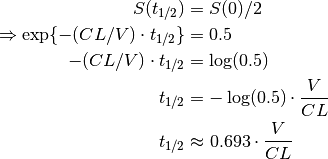
One quantity of interest in PK is half-life ( ), the time taken for drug concentration to fall to half that of its peak value. For a one compartment model with IV administration, we can calculate directly from the closed form solution:
Next, we turn to the case where the drug is administered via a route that requires absorption (i.e. anything except intravenous or intra-arterial injection).
One Compartment Model with Absorption
Many drugs are not administered directly into the bloodstream but are given orally, into the gastrointestinal tract, from which absorption must occur before the drug is observed in the plasma. Drugs are also frequently administered by other methods such as subcutaneously or intramuscularly, in which case absorption will also need to be modelled.
We model this using one or more absorption compartments (which we refer to as Depot compartments), connected via a one-way flow to the Central compartment.
Note
In PKPD terminology, the Depot compartment is not counted as a compartment, hence this is called a “one compartment model with absorption” even though it has two “compartments”.
Note
See the One Compartment Model with Absorption for Tut Script used to generate results in this section.
In a first order absorption model, the flow from the Depot to the Central compartment is proportional to the amount of drug in Depot, and the constant of proportionality is known as the absorption rate, KA:

Fig. 11 Compartment diagram for a one compartment model with absorption.
We must therefore model three flows:
- A bolus dose to the Depot
- A negative (outward) first order flow from the Depot with a rate constant of KA. This must be matched by a positive (inward) first order flow to the Central compartment.
- A negative (outward) flow from the Central compartment to account for elimination.
which we specify directly in the DERIVATIVES section of the PoPy script:
DERIVATIVES: |
    d[DEPOT]   = @bolus{amt:c[AMT]} - c[KA]*s[DEPOT]
    d[CENTRAL] = c[KA]*s[DEPOT] - c[CL]*s[CENTRAL]/c[V]
PoPy allows you to define the flows between compartments incrementally to simplify the model specification, after first initializing the flows to zero:
DERIVATIVES: |
    # initialize
    d[DEPOT]   = 0.0
    d[CENTRAL] = 0.0
    # update
    d[DEPOT] += @bolus{amt:c[AMT]}  # dose in
    d[DEPOT->CENTRAL] += c[KA]*s[DEPOT]  # absorption
    d[CENTRAL] -= c[CL]*s[CENTRAL]/c[V]  # elimination out
In this case, flows in from an external “source” are added using +=, flows out to an external “sink” are subtracted using -=, and flows between compartments are added using += with the arrow (->) notation to define the compartments being linked.
This notation has the advantage that the pairing of compartments is explicit and every flow is defined only once rather than having to maintain two equal and opposite flows, thus reducing the potential for human error when defining the model.
We note that, as in One Compartment Model with Intravenous Dosing, PoPy provides a closed form solution for this model:
DERIVATIVES: |
    s[DEPOT,CENTRAL] = @dep_one_cmp_cl{
        dose: @bolus{amt:c[AMT]},
        KA: c[KA], CL: c[CL], V: c[V]}
where dep (rather than iv) in the first part of the shortcut name denotes that a Depot compartment is included.

Fig. 12 Concentration vs Time curve for a one compartment model with absorption
Regardless of which formulation is used, the resulting Concentration vs Time curve is the same (Fig. 12). In this case, the amount of drug in Central rises more slowly than in the intravenous case as the drug is absorbed, peaks at a lower amount, then drops off at an approximately exponential rate as elimination removes the drug from the body.
Note
It is common for a drug to be absorbed more quickly than it is eliminated. In some cases, however, the opposite is true and the elimination rate becomes limited by the absorption rate (because in practice the drug cannot be eliminated faster than it is absorbed). This phenomenon is known as flip flop kinetics.
We now turn to the case where the drug diffuses at different rates between the blood and at least one other organ, modelled by adding a peripheral compartment.
Two Compartment Model
Two Compartment Model with Intravenous Dosing
For simplicity, we return to intravenous administration of the drug directly into the Central compartment. This time, however, we add a peripheral distribution compartment, Peri, that models the different distribution of the drug between the blood and/or well perfused organs and other tissues. The peripheral compartment is a useful approximation, which captures the impact of tissues with slower distribution on the shape of the plasma concentration-time profile.
Note
See the Two Compartment Model with Intravenous Dosing for Tut Script used to generate results in this section.
Because the diffusion can occur in both directions (unlike in absorption), we must now model the flow from Central to Peri and from Peri back to Central. We therefore introduce two new parameters:
- Q, the intercompartmental clearance
- V2, the volume of distribution of Peri (compartment 2)
and rename the volume of distribution of the Central compartment from V to V1 in order to distinguish it from that of the Peri compartment:

Fig. 13 Compartment diagram for a two compartment model with intravenous dosing.
The corresponding DERIVATIVES section is:
DERIVATIVES: |
    # initialize
    d[CENTRAL] = 0.0
    d[PERI] = 0.0
    # update
    d[CENTRAL] += @bolus{amt:c[AMT]}
    d[CENTRAL->PERI] += c[Q]*s[CENTRAL]/c[V1]  # intercompartmental diffusion
    d[PERI->CENTRAL] += c[Q]*s[PERI]/c[V2]  # intercompartmental diffusion
    d[CENTRAL] -= c[CL]*s[CENTRAL]/c[V1]
and, again, there is a convenient shortcut, @iv_two_cmp_cl
DERIVATIVES: |
    s[CENTRAL,PERI] = @iv_two_cmp_cl{
        dose: @bolus{amt:c[AMT]},
        CL: c[CL], V1: c[V1],
        Q: c[Q], V2: c[V2] }
As in previous examples, the resulting Concentration vs Time curve (Fig. 14) is the same regardless of whether we use flows or the closed form solution because they are equivalent.

Fig. 14 Concentration vs Time curve for a two compartment model with intravenous dosing
Two Compartment Model with Absorption
We can now model the effect of absorption (i.e. a Depot compartment), either by adding a Depot compartment to Two Compartment Model with Intravenous Dosing or by adding a Peri compartment to One Compartment Model with Absorption.
Note
See the Two Compartment Model with Absorption for Tut Script used to generate results in this section.

Fig. 15 Compartment diagram for a two compartment model with absorption
The resulting DERIVATIVES section is:
DERIVATIVES: |
    # initialize
    d[DEPOT]   = 0.0
    d[CENTRAL] = 0.0
    d[PERI] = 0.0
    # add flows
    d[DEPOT] += @bolus{amt:c[AMT]}
    d[DEPOT->CENTRAL] += c[KA]*s[DEPOT]  # absorption
    d[CENTRAL->PERI] += c[Q]*s[CENTRAL]/c[V]
    d[PERI->CENTRAL] += c[Q]*s[PERI]/c[V2]
    d[CENTRAL] -= c[CL]*s[CENTRAL]/c[V]
which also has a closed-form shortcut:
DERIVATIVES: |
    s[DEPOT,CENTRAL,PERI] = @dep_two_cmp_cl{
        dose: @bolus{amt:c[AMT]},
        KA: c[KA], CL: c[CL], V1: c[V1],
        Q: c[Q], V2: c[V2] }

Fig. 16 Concentration vs Time for a two compartment model with absorption
In the resulting Concentration vs Time curve (Fig. 16) we see a combination of the behaviours exhibited in the two earlier examples (Two Compartment Model with Intravenous Dosing and One Compartment Model with Absorption).
Three Compartment Model
Three Compartment Model with Intravenous Dosing
For completeness, we look at models with three compartments: the Central compartment and two peripheral compartments, Peri1 and Peri2.
Note
See the Three Compartment Model with Intravenous Dosing for Tut Script used to generate results in this section.
As in Two Compartment Model with Intravenous Dosing, we add two new parameters:
- Q3, the inter-compartmental clearance between Central and Peri2 (compartment 3)
- V3, the volume of distribution of Peri2 (compartment 3)
and rename the inter-compartmental clearance between Central and Peri1 (compartment 2) from Q to Q2.

Fig. 17 Compartment diagram for a three compartment model with intravenous dosing
After adding the two new flows to Peri2, the DERIVATIVES sections is now:
DERIVATIVES: |
    # initialize
    d[CENTRAL] = 0.0
    d[PERI1] = 0.0
    d[PERI2] = 0.0
    # update
    d[CENTRAL] += @bolus{amt:c[AMT]}  # dose in
    d[CENTRAL->PERI1] += c[Q2]*s[CENTRAL]/c[V1]
    d[PERI1->CENTRAL] += c[Q2]*s[PERI1]/c[V2]
    d[CENTRAL->PERI2] += c[Q3]*s[CENTRAL]/c[V1]
    d[PERI2->CENTRAL] += c[Q3]*s[PERI2]/c[V3]
    d[CENTRAL] -= c[CL]*s[CENTRAL]/c[V1]  # elimination out
and again there is a closed-form shortcut, iv_three_cmp_cl.
DERIVATIVES: |
    s[CENTRAL,PERI1,PERI2] = @iv_three_cmp_cl{
        dose: @bolus{lag:0, amt:c[AMT]},
        CL: c[CL], V1: c[V1],
        Q2: c[Q2], V2: c[V2],
        Q3:c[Q3], V3: c[V3] }
both of which give the same Concentration vs Time curve (Fig. 18), though it is not easy to see the impact of the second peripheral compartment that provides the transitional phase between the very steep initial fall and the shallow first-order terminal phase.

Fig. 18 Amount vs. Time for a three compartment model with intravenous dosing
Three Compartment Model with Absorption
The final model we consider in this chapter is a three compartment model with first order absorption (Fig. 19), specified either by adding a Depot compartment to Three Compartment Model with Intravenous Dosing or by adding a second peripheral compartment to Two Compartment Model with Absorption.
Note
See the Three Compartment Model with Absorption for Tut Script used to generate results in this section.

Fig. 19 Compartment diagram for a three compartment model with absorption
The DERIVATIVES section,
DERIVATIVES: |
    # initialize
    d[DEPOT] = 0.0
    d[CENTRAL] = 0.0
    d[PERI1] = 0.0
    d[PERI2] = 0.0
    # update
    d[DEPOT] += @bolus{amt:c[AMT]} # dose in
    d[DEPOT->CENTRAL] += c[KA]*s[DEPOT]  # absorption
    d[CENTRAL->PERI1] += c[Q2]*s[CENTRAL]/c[V1]
    d[PERI1->CENTRAL] += c[Q2]*s[PERI1]/c[V2]
    d[CENTRAL->PERI2] += c[Q3]*s[CENTRAL]/c[V1]
    d[PERI2->CENTRAL] += c[Q3]*s[PERI2]/c[V3]
    d[CENTRAL] -= c[CL]*s[CENTRAL]/c[V1]  # elimination out
also has a closed form shortcut,
DERIVATIVES: |
    s[DEPOT,CENTRAL,PERI1,PERI2] = @dep_three_cmp_cl{
        dose: @bolus{lag:0, amt:c[AMT]},
        KA: c[KA], CL: c[CL], V1: c[V1],
        Q2: c[Q2], V2: c[V2],
        Q3: c[Q3], V3: c[V3]}
both of which produce the same Concentration vs Time curve, which resembles that from Two Compartment Model with Absorption only with a lower peak (Fig. 20).

Fig. 20 Concentration vs Time for a three compartment model with absorption