Fitting a Two Compartment PopPK Model
The Fitting a Simple PopPK Model using PoPy shows fitting a one compartment PK model, to pre-existing data. In this example, we again utilise a pre-existing data set. We will demonstrate how to fit a two compartment model with absorption and bolus dosing, see Fig. 40:-

Fig. 40 Two compartment model with depot dosing for Fit Script. Here c[AMT] is the size of the bolus dose specified in the data file. m[KA], m[CL], m[Q], m[V1], m[V2] are all MODEL_PARAMS to be estimated for each individual.
This model is called a two compartment model, because the Depot is not included, only the compartments that conventionally represent blood volumes are counted. In this case Central and Peri.
This PoPy model is also created by default when Creating an example Fit Script, using popy_create.
Note
See the First order absorption model with peripheral compartment obtained by the PoPy developers for this example, including input script and input data file.
Run the Fit Script
This fitting example uses these two files:-
c:\PoPy\examples\builtin_fit_example.pyml
                 builitin_fit_example_data.csv
Open a PoPy Command Prompt to setup the PoPy environment in this folder:-
c:\PoPy\examples\
With the PoPy environment enabled, do:-
$ popy_edit builtin_fit_example.pyml
To view the script in an editor and then run the Fit Script using popy_run from the command line:-
$ popy_run builtin_fit_example.pyml
When the fit script has completed, you can view the output of the fit using popy_view, by typing the following command:-
$ popy_view builtin_fit_example.pyml.html
Note the extra ‘.html’ extension in the above command. This command opens a local .html file in your web browser to summarise the result of the fitting.
You can compare your local html output with the pre-computed documentation output, see First order absorption model with peripheral compartment. You should expect some minor numerical differences when comparing results with the documentation.
Summary of Fit Results
The results of running the fitting script are PoPy’s best estimate for the presumed unknown fixed effects variables:-
f[KA] = 0.2115
f[CL] = 2.0587
f[V1] = 53.0562
f[Q] = 0.9970
f[V2] = 104.3821
f[KA_isv,CL_isv,V1_isv,Q_isv,V2_isv] = [
    [ 0.1078, 0.0156, -0.0551, 0.0615, -0.0371 ],
    [ 0.0156, 0.0658, 0.0054, -0.0648, -0.0879 ],
    [ -0.0551, 0.0054, 0.0535, -0.0610, 0.0215 ],
    [ 0.0615, -0.0648, -0.0610, 0.3495, 0.0985 ],
    [ -0.0371, -0.0879, 0.0215, 0.0985, 0.1857 ]
]
f[PNOISE] = 0.1415
The aim of a Fit Script is to optimise the fixed effects and random effects maximizing the likelihood of observing the input data given the model structure defined in ‘builtin_fit_example.pyml’. The input data in this case, is the c[DV_CENTRAL] column in ‘builtin_fit_example_data.csv’, which contains 50 individuals each with 5 observations at random time points following a bolus dose event.
You can visually compare the initial f[X] and fitted f[X] outputs with the input data, see Table 23.

|
|

|
In the graphs above the blue dots represent the original data points. The solid blue line represents the model predictions given the final f[X] parameters and fitted r[X] values for each individual. The dashed blue lines represent the model predictions given initial f[X] parameters and r[X] values set to zero.
Note in this model a bolus dose is received by all individuals at time 2.0. Then the amount of drug in the Central compartment follows a complex PK curve as it is first absorbed form the Depot compartment and then eliminated over time, whilst also interacting with the Peripheral compartment.
The graphs show that PoPy has adjusted the f[X] and r[X] parameters, so that the PK curves more closely match the input data and therefore maximise the likelihood of the data being generated from this model.
The data file included in this example is synthesized from the PK model of the same form described in ‘builtin_fit_example.pyml’ (see Generate a Two Compartment PopPK Data Set). So in this case, the model structure is known to be correct, so we should expect a good model fit.
Syntax of Fit Script
The mixed effect population structure is defined in the EFFECTS section as follows:-
EFFECTS:
    POP: |
        f[KA] ~ P1.0
        f[CL] ~ P1.0
        f[V1] ~ P20
        f[Q] ~ P0.5
        f[V2] ~ P100
        f[KA_isv,CL_isv,V1_isv,Q_isv,V2_isv] ~ spd_matrix() [
            [0.05],
            [0.01, 0.05],
            [0.01, 0.01, 0.05],
            [0.01, 0.01, 0.01, 0.05],
            [0.01, 0.01, 0.01, 0.01, 0.05],
        ]
        f[PNOISE] ~ P0.1
    ID: |
        r[KA, CL, V1, Q, V2] ~ mnorm([0,0,0,0,0], f[KA_isv,CL_isv,V1_isv,Q_isv,V2_isv])
There are 5 mean fixed effect parameters i.e. f[KA], f[CL], f[V1], f[Q], f[V2], a 5x5 covariance matrix f[KA_isv, CL_isv, V1_isv, Q_isv, V2_isv], a proportional noise variable f[PNOISE] and a 5 element vector r[KA, CL, V1, Q, V2] of random effects defined for each individual. There are 50 individuals in the data set, therefore this model is attempting to estimate 6 main f[X] parameters, 15 variance f[X] parameters (the covariance matrix is symmetric) and 5 r[X] per individual. There are 271 parameters in total (i.e 15+6 f[X] + 50*5 r[X]).
The allowable ranges and starting values for the main f[X] are defined using the following syntax:-
f[X] ~ P start_x
Here the ‘P’ is short for ‘positive’. This expression is actually a shortcut for:-
f[X] ~ unif(0.0, +inf) start_x
Where a ~unif() distribution is used to define a range of allowed values [0.0, +inf]. Note, it’s quite common to require PK/PD model parameters be non-negative, in order to make physical sense. The ‘start_x’ value is the initial value for f[X] used in the optimisation, which is usually an initial guess by the modeller.
Each individual has a unique r[KA, CL, V1, Q, V2] vector, because the random effects are defined at the ID level. For more info on the syntax above see EFFECTS. The r[X] are here defined as a zero-mean, multi-variate normal distribution:-
r[KA, CL, V1, Q, V2] ~ mnorm([0,0,0,0,0], f[KA_isv,CL_isv,V1_isv,Q_isv,V2_isv])
Note the second parameter of ~mnorm() distribution, the square covariance matrix f[KA_isv, CL_isv, V1_isv, Q_isv, V2_isv] is a population parameter shared by all individuals.
When fitting a model, the f[KA_isv, CL_isv, V1_isv, Q_isv, V2_isv] matrix is defined using a ~spd_matrix() distribution:-
f[KA_isv,CL_isv,V1_isv,Q_isv,V2_isv] ~ spd_matrix() [
    [0.05],
    [0.01, 0.05],
    [0.01, 0.01, 0.05],
    [0.01, 0.01, 0.01, 0.05],
    [0.01, 0.01, 0.01, 0.01, 0.05],
]
Where spd is short for symmetric positive definite. This distribution will always return a matrix with positive eigenvalues, starting with an initial matrix:-
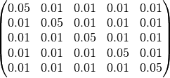
Note as the initial matrix is symmetric it is only necessary to specify the lower triangle elements. PoPy will update the 15 free elements of this matrix to increase the likelihood fit.
Given the f[X] and r[X] the mapping to the m[X] for each individual is defined in the MODEL_PARAMS section:-
MODEL_PARAMS: |
    m[KA] = f[KA] * exp(r[KA])
    m[CL] = f[CL] * exp(r[CL])
    m[V1] = f[V1] * exp(r[V1])
    m[Q] = f[Q] * exp(r[Q])
    m[V2] = f[V2] * exp(r[V2])
    m[ANOISE] = 0.001
    m[PNOISE] = f[PNOISE]
This shows that the m[KA], m[CL], m[V1], m[Q], m[V2] parameters for each individual are modelled as log normal distributions with median values of f[KA], f[CL], f[V1], f[Q], f[V2]. There is a shared proportional noise parameter f[PNOISE] for all individuals. And small fixed additive noise constant m[ANOISE]. For more info on the syntax above see MODEL_PARAMS.
A two compartment model with first order elimination and bolus dosing via a depot compartment is defined in the DERIVATIVES section:-
DERIVATIVES: |
    # s[DEPOT,CENTRAL,PERI] = @dep_two_cmp_cl{dose:@bolus{amt:c[AMT]}}
    d[DEPOT] = @bolus{amt:c[AMT]} - m[KA]*s[DEPOT]
    d[CENTRAL] = m[KA]*s[DEPOT] - s[CENTRAL]*m[CL]/m[V1] - s[CENTRAL]*m[Q]/m[V1]  + s[PERI]*m[Q]/m[V2]
    d[PERI] = s[CENTRAL]*m[Q]/m[V1] - s[PERI]*m[Q]/m[V2]
The bolus arrives in the Depot compartment, due to the @bolus term appearing on the right hand side of the d[DEPOT] equation:-
d[DEPOT] = @bolus{amt:c[AMT]} - m[KA]*s[DEPOT]
The amount of the bolus dose is c[AMT], which is defined in the data file. In this case it is always 100 units and occurs at time point 2.0 for all individuals. The elimination rate from the Depot compartment is m[KA], which is first order with respect to s[DEPOT].
The Central compartment, which represents the blood plasma and where drug concentration observations are made is defined as follows:-
d[CENTRAL] = m[KA]*s[DEPOT] - s[CENTRAL]*m[CL]/m[V1] - s[CENTRAL]*m[Q]/m[V1] + s[PERI]*m[Q]/m[V2]
This consists of the input from the Depot m[KA]*s[DEPOT] and a first order elimination expression s[CENTRAL]*m[CL]/m[V1] that represents the removal of the drug from the blood plasma. Here the elimination rate is expressed as a ratio of:-
m[CL]: clearance from Central compartmentm[V1]: volume of distribution of Central compartment
The last two terms - s[CENTRAL]*m[Q]/m[V1] + s[PERI]*m[Q]/m[V2] are simply the negative values of the rates for the Peripheral compartment:-
d[PERI] = s[CENTRAL]*m[Q]/m[V1] - s[PERI]*m[Q]/m[V2]
To compute the objective function for each row of the data set, the s[X] values are used to compute p[X] prediction variables which are then compared with the target c[X] values from the data file, as defined below:-
PREDICTIONS: |
    p[CEN] = s[CENTRAL]/m[V1]
    var = m[ANOISE]**2 + m[PNOISE]**2 * p[CEN]**2
    c[DV_CENTRAL] ~ norm(p[CEN], var)
The predicted variable p[CEN] is defined as follows:-
p[CEN] = s[CENTRAL]/m[V1]
Hence this is a concentration, because we are dividing the amount s[CENTRAL] by the volume of distribution of the Central compartment. The other two lines:-
var = m[ANOISE]**2 + m[PNOISE]**2 * p[CEN]**2
c[DV_CENTRAL] ~ norm(p[CEN], var)
show that we are comparing the model prediction p[CEN] with the data c[DV_CENTRAL] and using ~norm() distribution likelihood error model. The variance is a proportional noise model, where the standard deviation of the proportional noise is m[PNOISE]. Here m[ANOISE] is fixed to a small positive constant, this is to avoid zero variances when p[CEN] is close to zero. For more info on the syntax above see PREDICTIONS.
PoPy is essentially trying to find the best combination of fixed parameters as follows:-
f[KA]- the median elimination rate from the Depot -> Central compartmentf[CL]- the median clearance of the Central compartmentf[V1]- the median volume of distribution of the Central compartmentf[Q]- the median clearance between the Central <-> Peripheral compartmentsf[V2]- the median volume of distribution of the Peripheral compartmentf[KA_isv, CL_isv, V1_isv, Q_isv, V2_isv]- The covariance structure of thef[X]parameters above over the population of individuals.f[PNOISE]- the proportional noise not explained by the model in thec[DV_CENTRAL]data.
The unexplained noise f[PNOISE] and between subject variance f[KA_isv, CL_isv, V1_isv, Q_isv, V2_isv] obfuscate each other. However the population as a whole contains enough data to solve this problem using maximum likelihood [Sheiner1980].
In PoPy the likelihood is optimised iteratively, with the f[X] and r[X] being updated at each iteration. In this case, the likelihood (or objective function) progressed as follows (Table 24):
| Iteration | Time | OBJV |
| 0 | 0.72 | 4694.97944955 |
| 1 | 3.82 | 925.406423154 |
| 2 | 4.10 | 925.406423154 |
| 3 | 8.28 | -665.711652792 |
| 4 | 12.56 | -793.296791963 |
| 5 | 15.91 | -852.722217074 |
| 6 | 18.85 | -877.656289502 |
| 7 | 21.50 | -884.987157492 |
| 8 | 24.21 | -887.327506213 |
| 9 | 26.71 | -888.347860221 |
| 10 | 29.19 | -888.945264113 |
| 11 | 31.77 | -889.409728315 |
| 12 | 34.45 | -889.875813598 |
| 13 | 37.01 | -890.548536936 |
| 14 | 39.59 | -891.812439894 |
| 15 | 42.11 | -892.731368384 |
| 16 | 44.89 | -893.230662133 |
| 17 | 47.71 | -893.629616339 |
| 18 | 50.43 | -894.034893077 |
| 19 | 53.16 | -894.454077437 |
| 20 | 55.82 | -894.877997128 |
| 21 | 58.38 | -895.310624973 |
| 22 | 61.01 | -895.727031561 |
| 23 | 63.70 | -896.131448931 |
| 24 | 66.36 | -896.52824934 |
| 25 | 69.09 | -896.908775406 |
| 26 | 71.73 | -897.272108888 |
| 27 | 74.41 | -897.617172046 |
| 28 | 77.04 | -897.939699429 |
| 29 | 79.79 | -898.230353198 |
| 30 | 82.52 | -898.489898229 |
| 31 | 85.29 | -898.709767912 |
| 32 | 88.08 | -898.89080333 |
| 33 | 90.04 | -898.89080336 |
Note that the objective function is defined as -2 * the log likelihood. Therefore the lower the objective function the more likely the input data will be observed given the current f[X] values. By default PoPy stops the fitting algorithm once the objective function has stopped decreasing.
Visual Predictive Check for Two Compartment PopPK Model
The Fitting a Two Compartment PopPK Model section showed fitting a PK/PD model to a data set.
As shown previous in Visual Predictive Check for Simple PopPK Model. It is possible to use the fitted fixed effects values, i.e the optimised f[X] variables, to generate a visual predictive check, often abbreviated to ‘VPC’.
Running the MSim Script
It is presumed that you have already run the ‘builtin_fit_example.pyml’ script from Fitting a Two Compartment PopPK Model. If you have then you should have access to the following output folder:-
builtin_fit_example.pyml_output/
    msim/
        builtin_fit_example_msim.pyml
You need to Open a PoPy Command Prompt in the ‘msim’ sub folder then do:-
$ popy_edit builtin_fit_example_msim.pyml
To open the MSim Script in an editor. You can then run the script using:-
$ popy_run builtin_fit_example_msim.pyml
If you run this script the following .svg file is output:-
builtin_fit_example_msim.pyml_output/
    DV_CENTRAL_sim,DV_CENTRAL_wrt_TIME_SINCE_LAST_DOSE_comb_quant_sim_vpc/
        000000.svg
This graphic should look something like Fig. 41:-

Fig. 41 Visual Predictive Check for Complex PopPK model.
Here the y axis is the concentration in the Central compartment and the x axis is the time since the last dose (TSLD). See Visual Predictive Check for Simple PopPK Model for a more general description of the VPC plot shown in Fig. 41.
In this case, the TSLD values are grouped into 12 equally spaced bins along the x axis. Note you need a minimum number of data points in each bin and there are only 250 data points in this toy example. Hence the small number of bins.
The blue dots (original data) are mainly shown to give some visual corroboration of the quantiles (solid blue line). In this graph there are only 12 bins and therefore each bin is quite wide, therefore some data points are grouped together inappropriately. This grouping issue is most obvious at the smaller values of TSLD, during the drug uptake period, when the drug is being mainly absorbed into Central compartment and has not been cleared from the blood plasma yet (see Fig. 41). Only more data and more bins can really fix the issue.
Syntax in the MSim Script
For each individual in the original data set, new synthetic data sets are created by sampling new random effects r[X] variables and new measurement noise for all data rows. i.e. The synthetic populations vary due to sampling the r[X] for each individual here:-
EFFECTS:
    ID: |
        r[KA, CL, V1, Q, V2] ~ mnorm([0,0,0,0,0], f[KA_isv,CL_isv,V1_isv,Q_isv,V2_isv])
And adding measurement noise here:-
PREDICTIONS: |
    p[CEN_sim] = s[CENTRAL]/m[V1]
    var = m[ANOISE]**2 + m[PNOISE]**2 * p[CEN_sim]**2
    c[DV_CENTRAL_sim] ~ norm(p[CEN_sim], var)
This procedure creates a set of N new data sets, which can be compared with the original data set. Where N is defined here:-
OUTPUT_OPTIONS:
    n_pop_samples: 100
You can increase the number of samples, to make the VPC more representative of your model. The more complex the PK/PD model, the more synthetic data samples you will need.
As this model has more parameters compared to the Fitting a Simple PopPK Model using PoPy, it may be worth increasing the ‘n_pop_samples’ and re-running the MSim Script. This is left as an exercise for the reader.