Residual Error Model
So far, we have looked at compartment models and different dosing regimes all under theoretical conditions. For example, our Concentration vs Time curve for a one compartment model with absorption produces smooth curves with evenly spaced observation points (Fig. 26).

Fig. 26 Concentration vs Time for a one compartment model with absorption, without measurement error (noise).
In practice, however, it is impossible to measure any quantity perfectly; all measurements are imperfect and contain some noise. To weight each observation correctly, we may need to account for patterns of noise in the data. For example, noise often increases proportionally with signal so that higher concentrations contain more absolute error. Sometimes we know that observations have been collected in suboptimal conditions and may wish to allow the model to downweight them if they are inconsistent with other data.
We therefore turn to the different ways in which noise manifests itself on the observations and how we can incorporate this into a fitted model.
Error Models for Continuous Data
Specifically, we look at how to model errors that appear on a continuous quantity such as the measured concentration of drug, demonstrating the concept using a normal distribution (a popular choice for continuous measurements).
Additive Noise
Note
See the Model containing additive error only and additive error only input data for the Tut Script used to generate results in this section.
In the simplest case, the difference between the observed measurement and the model prediction will be a random variable of constant variance (or, equivalently, constant standard deviation) such that the observations are scattered evenly around the ideal curve.
PREDICTIONS: |
    plabel[DV_CENTRAL] = "Drug Concentration (mg/L)"
    clabel[TIME] = "Time (minutes)"
    p[DV_CENTRAL] = s[CENTRAL]/m[V]
    add_std = m[ANOISE_STD]
    total_var = add_std**2
    c[DV_CENTRAL] ~ norm(p[DV_CENTRAL], total_var)
With a standard deviation of 1.0, for example, and 100 randomly sampled time points between 1 and 40, we get a more realistic Concentration vs Time curve (Fig. 27).

Fig. 27 Concentration vs Time for a one compartment model with absorption, plus additive noise.
Proportional Noise
Note
See the Model containing proportional error only, with proportional only data for the Tut Script used to generate results in this section.
While additive noise is independent of the strength of the signal (e.g. the magnitude of the measurement) at any point in time, proportional noise increases in proportion to the magnitude of the signal. For example, the standard deviation of the noise may be equal to 10% of the signal magnitude such that the error is greatest at the peak of the curve, reducing as the concentration falls (Fig. 28)
PREDICTIONS: |
    plabel[DV_CENTRAL] = "Drug Concentration (mg/L)"
    clabel[TIME] = "Time (minutes)"
    p[DV_CENTRAL] = s[CENTRAL]/m[V]
    prop_std = p[DV_CENTRAL] * m[PNOISE_STD]
    total_var = prop_std**2
    c[DV_CENTRAL] ~ norm(p[DV_CENTRAL], total_var)

Fig. 28 Concentration vs Time for a one compartment model with absorption, plus proportional noise.
Additive and Proportional Noise
Note
See the Model containing both proportional and additive error for the Tut Script used to generate results in this section.
In reality, most measurement processes are affected by both kinds of error such that the additive noise dominates at low signal magnitudes whereas proportional noise dominates at high signal magnitudes (Fig. 29).

Fig. 29 Concentration vs Time for a one compartment model with absorption, plus both proportional and additive noise
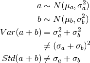
We must, however, take care when defining the variance of a mixed error model. The variance of the sum of two normally distributed variables is the sum of their variances, and therefore the standard deviation of the sum does not equal the sum of their standard deviations:
as shown in the PREDICTIONS block of the PoPy input script:
PREDICTIONS: |
    plabel[DV_CENTRAL] = "Drug Concentration (mg/L)"
    clabel[TIME] = "Time (minutes)"
    p[DV_CENTRAL] = s[CENTRAL]/m[V]
    prop_std = p[DV_CENTRAL] * m[PNOISE_STD]
    add_std = m[ANOISE_STD]
    total_var = prop_std**2 + add_std**2
    c[DV_CENTRAL] ~ norm(p[DV_CENTRAL], total_var)
It is crucially important to specify the form of the total variance correctly when fitting if we are to estimate the additive and proportional variances correctly. To see the effect of specifying the variance incorrectly, compare the tutorial script Mixed error model fitted to mixed error data, but with incorrect variance definition with its correct counterpart, Model containing both proportional and additive error.