Matrices
The matrices available for use in PoPy models are shown in Table 68:-
| Name | Syntax |
|---|---|
| Constant Diagonal Matrix | y_mat = [[x(1,1), x(2,2)]] |
| Constant Square Matrix | y_mat = [[x(1,1)], [x(2,1), x(2,2)]] |
| SPD Diagonal Matrix | y_mat ~ diag_matrix() [[x(1,1), x(2,2)]] |
| SPD Square Matrix | y_mat ~ spd_matrix() [[x(1,1)], [x(1,2), x(2,2)]] |
Constant Diagonal Matrix
A constant nxn diagonal matrix is specified using the following syntax:-
y_mat = [[x(1,1), x(2,2), ... , x(n,n)]]
Where:-
- y_mat is a multi-element
f[X]matrix label - x(1,1) is the first element of the diagonal
- x(n,n) is the last element of the diagonal
Note
A diagonal matrix definition in PoPy starts with double opening square brackets ‘[[‘ and ends with matching double closing square brackets ‘]]’.
This is to distinguish from a list which uses single square brackets.
An example diagonal matrix is shown below:-
f[KA_isv,CL_isv,V1_isv,Q_isv,V2_isv] = [
        [ 0.1, 0.03, 0.09, 0.07, 0.05]
    ]
Here a 5x5 matrix called f[KA_isv, CL_isv, V1_isv, Q_isv, V2_isv] is created with the following values:-
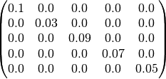
In the definition above the number of f[X] labels on the left hand side must correspond to the number of list elements along the diagonal on the right hand side. i.e. in this case they both contain 5 elements.
Constant Square Symmetric Matrix
A constant nxn square symmetric matrix is specified using the following syntax:-
y_mat = [
    [x(1,1)],
    [x(2,1), x(2,2)],
    ...
    [x(n,1), x(n,2) ... , x(n,n)]
]
Where:-
- y_mat is a multi-element
f[X]matrix label - x(1,1) is the first element of the diagonal
- x(i,j) defines the element of the ith row and jth column
- x(n,n) is the last element of the diagonal
The definition above just requires the lower triangular elements to be defined, because the matrix is assumed to be square and symmetric.
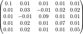
An example of defining a square symmetric matrix is shown below:-
f[KA_isv,CL_isv,V1_isv,Q_isv,V2_isv] = [
        [0.1],
        [0.01, 0.03],
        [0.01, -0.01, 0.09],
        [0.01, 0.02, 0.01, 0.07],
        [0.01, 0.02, 0.01, 0.01, 0.05],
    ]
The number of elements in each row of the matrix definition need to be [1,2,3,4,5], because the f[X] variable contains 5 elements.
Therefore a 5x5 matrix called f[KA_isv, CL_isv, V1_isv, Q_isv, V2_isv] is created with the following values:-
Note you can also define the same matrix as follows:-
f[KA_isv,CL_isv,V1_isv,Q_isv,V2_isv] = [
        [0.1 , 0.01,  0.01, 0.01, 0.01],
        [0.01, 0.03, -0.01, 0.02, 0.02],
        [0.01, -0.01, 0.09, 0.01, 0.01],
        [0.01, 0.02,  0.01, 0.07, 0.01],
        [0.01, 0.02,  0.01, 0.01, 0.05],
    ]
However this format risks accidentally creating a non-symmetric matrix.
In PoPy, you can only specify square symmetric matrices. If the input matrix is non-square PoPy will report an error. If the input matrix is square, but non-symmetric then PoPy will average the upper and lower triangles and output a warning.
Positive Definite Diagonal Matrix
A positive definite nxn diagonal matrix for estimation is specified using the following syntax:-
y_mat ~ diag_matrix() [[x(1,1), x(2,2), ... , x(n,n)]]
Where:-
- y_mat is a multi-element
f[X]matrix label - x(1,1) is the first element of the diagonal
- x(n,n) is the last element of the diagonal
Note
The ‘~’ notation means that ‘y_mat’ is a diagonal matrix to be estimated, and only initialised with the diagonal matrix specified in square brackets.
An example diagonal matrix for estimation in a Fit Script is shown below:-
f[KA_isv,CL_isv,V1_isv,Q_isv,V2_isv] ~ diag_matrix() [
        [ 0.1, 0.03, 0.09, 0.07, 0.05]
    ]
Here a 5x5 matrix variable f[KA_isv, CL_isv, V1_isv, Q_isv, V2_isv] is initialised with the following values:-
In the fitting process the diagonal elements are constrained to be positive and the off diagonal terms are fixed to zero.
Note
This matrix is defined using the ‘~’ notation, however it is not a true distribution in the sense that if you sample from the matrix distribution, only the current value is returned. This fact is only relevant for a Gen Script or MGen Script.
Symmetric Positive Definite Matrix
A symmetric positive definite nxn square symmetric matrix for estimation is specified using the following syntax:-
y_mat ~ spd_matrix() [
    [x(1,1)],
    [x(2,1), x(2,2)],
    ...
    [x(n,1), x(n,2) ... , x(n,n)]
]
Where:-
- y_mat is a multi-element
f[X]matrix label - x(1,1) is the first element of the diagonal
- x(i,j) defines the element of the ith row and jth column
- x(n,n) is the last element of the diagonal
An example of defining a square symmetric matrix to be estimated is shown below:-
f[KA_isv,CL_isv,V1_isv,Q_isv,V2_isv] ~ spd_matrix() [
        [0.1],
        [0.01, 0.03],
        [0.01, -0.01, 0.09],
        [0.01, 0.02, 0.01, 0.07],
        [0.01, 0.02, 0.01, 0.01, 0.05],
    ]
Here we are only defining the lower triangle elements, as the upper triangle elements are the same in a symmetric matrix. The number of elements in each row of the initial matrix definition needs to be [1,2,3,4,5], because the f[X] variable contains 5 elements.
We are declaring a 5x5 matrix called f[KA_isv, CL_isv, V1_isv, Q_isv, V2_isv], that will be estimated by a Fit Script and is constrained to be symmetric positive definite. The matrix is initialised with the following values:-
Note that the symmetric ~spd_matrix() distribution is initialised here by defining just the lower triangular elements (without loss of generality), but it can also be initialised by carefully defining all 5*5 elements.
Covariance Matrix Usage
The most common use for matrices as defined above is to define a covariance matrix for a Multivariate Normal Distribution. For example in a EFFECTS section:-
EFFECTS:
    ID: |
        r[KA,CL,V1,Q,V2] ~ mnorm(
            [0, 0, 0, 0, 0], f[KA_isv,CL_isv,V1_isv,Q_isv,V2_isv] )
Here the matrix f[KA_isv, CL_isv, V1_isv, Q_isv, V2_isv], can be defined in any of the ways specified above, i.e. constant/variable or square/diagonal.
In the definition of r[KA, CL, V1, Q, V2], the size of the variance matrix must agree with the size of the random vector and the mean vector of the ~mnorm() distribution. See Multivariate Normal Random Effect Example for more information.