- Language: en
- Documentation version: 1.3.1
Infusion
An infusion administers the dose gradually, usually at a fixed rate over a fixed period of time (i.e. the rate of infusion is constant during the time period and zero before and after, typically intravenously).
The mathematical expression for an infusion is:
![\text{d[CENTRAL]} = \text{d[CENTRAL]} + \text{R(t)}](../../../_images/math/7e8020f2564cd7715b0c53eae04f506b204de617.png)
where the infusion has constant rate c[RATE], starts at time t=0 and has duration c[DUR] and in compartment CENTRAL is:-
where:-
![R(t)=
\Biggl \lbrace
{
c[RATE] ,\text{ if } { t_S \leq t \leq t_S + c[DUR] }
\atop
0.0, \text{ otherwise }
}](../../../_images/math/75912f9207216698c3006920db36c8c5db792658.png)
An infusion dose can be characterised either by the duration of the infusion or the rate of the infusion. As the rate of change is constant, an infusion is also known as zero order absorption.
Note: For a constant total infusion amount (AMT) the RATE and DURATION can be calculated from each other:

So specifying either a RATE or DURATION, together with a total amount, is sufficient to fully define an infusion.
Infusion Duration
An infusion duration is coded by:
@inf_dur{amt: c[AMT], lag: m[LAG], dur: c[DUR]}
in the equation for the appropriate compartment in the DERIVATIVES: section of a fit or tutorial script.
Dose and lag are coded in the same way as for a bolus dose.
Duration can either be included in the input data or can be estimated as a parameter.
Note
See the Infusion Duration Dose with no elimination. for Tut Script used to generate results in this section.
An example of an infusion dose spread over 20 time units added to a one compartment model with no lag time is:
DERIVATIVES: |
    d[CENTRAL] = (
        @inf_dur{amt: c[AMT], lag: 0.0, dur: 20}
        - m[KE]*s[CENTRAL]
    )
If the infusion duration varies between individuals use:
DERIVATIVES: |
    d[CENTRAL] = (
        @inf_dur{amt: c[AMT], lag: 0.0, dur: c[DUR]}
        - m[KE]*s[CENTRAL]
    )
See @inf_dur for some more syntax examples.
The Amount-vs-Time curve for an infusion (without elimination) is a ramp function where the cumulative dose rises linearly until it reaches the total amount administered (Fig. 5).
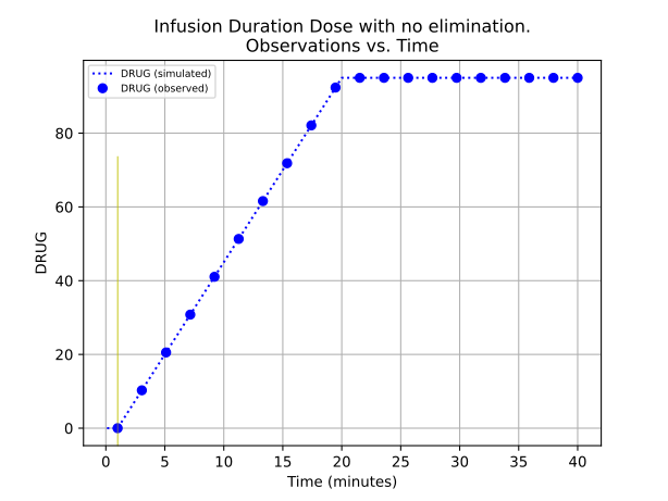
Fig. 5 Cumulative amount following a infusion dose of 95 mg over a duration of 19 min with no elimination
Infusion Rate
An infusion duration is coded by:
@inf_rate{amt: c[AMT], lag: m[LAG], rate: c[RATE]}
in the equation for the appropriate compartment in the DERIVATIVES: section of a fit or tutorial script.
The amount and lag are coded in the same way as for a bolus dose.
Infusion rate can either be included in the input data or can be estimated as a parameter.
Note
See the Infusion Rate Dose with no elimination. for Tut Script used to generate results in this section.
An example of an infusion dose at a rate of 5 dose units per time unit added to a one compartment model with no lag time is:
DERIVATIVES: |
    d[CENTRAL] = (
        @inf_rate{amt: c[AMT], lag: 0.0, rate: 5}
        - m[KE]*s[CENTRAL]
    )
If the infusion rate is different between individuals use:
DERIVATIVES: |
    d[CENTRAL] = (
        @inf_rate{amt: c[AMT], lag: 0.0, rate: c[RATE]}
        - m[KE]*s[CENTRAL]
    )
See @inf_rate for some more syntax examples.
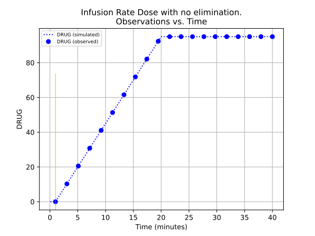
Fig. 6 Cumulative amount following a infusion dose of 95 mg at a rate of 5 mg/min with no elimination