Time Delay

In an indirect model there is a time delay between the drug concentration and the PD response due to the intermediate processes. There may also be a time delay in a direct response because the concentration of drug in the plasma may not be the same as the concentration at the site of the response.

Direct Effect Models

A direct response means that the drug has a direct effect on a PD process. For example, as levels of Quinidine increase, the length of the Q-T interval increases.

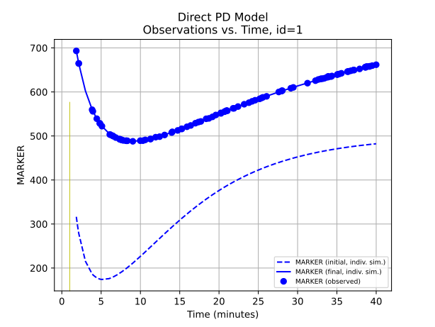
Direct PD Model is an example of a tutorial script of a simple direct PD model. The pharmacokinetic model is a one compartment model. Values of c[K] for each individual are simulated in the gen_params section. In a real world situation, the values of K would have been estimated by a previous pharmacokinetic model. The amount of drug in the CENTRAL compartment affects the rate at which the MARKER is removed from the system.

This is implemented in the DERIVATIVES section in the script script as shown below:

DERIVATIVES: |
    d[CENTRAL] = @bolus{amt:c[AMT]} - s[CENTRAL]*c[CL]/c[V]
    d[MARKER] = m[BASE]*m[KOUT] - (1+s[CENTRAL]/c[V])*m[KOUT]*s[MARKER]

Note that the following states section is also required to initialise the s[MARKER] value at the steady state concentration at time zero:

STATES: |
    s[CENTRAL] = 0.0
    s[MARKER] = m[BASE]

With these initial conditions d[MARKER] =0. s[MARKER] will only change if the drug is administered.

A compartment diagram of this model is shown below:

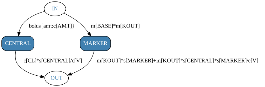
In contrast to the pharmacokinetic models, there is no actual movement between the compartments. The amount in the CENTRAL compartment just has an effect on the KOUT of the MARKER compartment.

Indirect Effect Models

In an indirect response PD Model the drug will affect an inter-mediate process, which then influences the measured PD response. A classic example is warfarin. Warfarin inhibits the synthesis of prothrombin, which in turn inhibits the formation of blood clots.

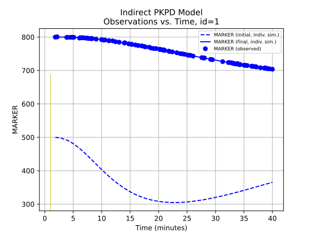
Indirect PKPD Model is a similar model, which includes a time delay in the effect on the MARKER compartment. This is achieved by two lag compartments, delaying the drug effect:

DERIVATIVES: |
    d[CENTRAL] = @bolus{amt:c[AMT]} - c[CL]*s[CENTRAL]/c[V]
    d[LAG1] = m[KOUT]*s[CENTRAL]/c[V] - m[KOUT]*s[LAG1]
    d[LAG2] = m[KOUT]*s[LAG1] - m[KOUT]*s[LAG2]
    d[MARKER] = m[BASE]*m[KOUT] - (1+s[LAG2])*m[KOUT]*s[MARKER]

As in the direct model, the initial steady state is achieved as follows:

STATES: |
    s[CENTRAL] = 0.0
    s[MARKER] = m[BASE]

The actual processes that occur between the CENTRAL compartment and the MARKER compartment are NOT modelled directly because we want to model a time delay and then the eventual effect of the amount in the CENTRAL compartment on the MARKER compartment clearance. A compartment diagram of this model is shown below:

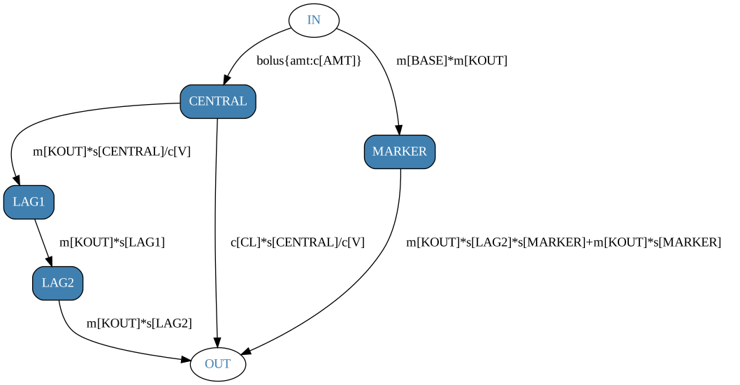
This is similar to Direct Effect Models, except that the effect of the amount in the CENTRAL compartment on the MARKER compartment is delayed by passing through the two lag compartments.

Linear Effect Model

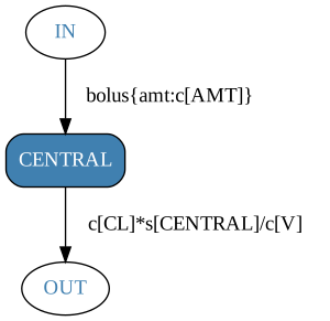
Linear PD model is a direct effect model where the PD Marker response is much simpler. The derivatives block is a standard one compartment PK model a follows:

DERIVATIVES: |
    d[CENTRAL] = @bolus{amt:c[AMT]} - c[CL]*s[CENTRAL]/c[V]

Resulting in the following compartment diagram:

The linear effect is defined in the predictions block as follows:

PREDICTIONS: |
    clabel[TIME] = "Time (minutes)"
    plabel[MARKER] = "Biomarker concentration (mg/L)"
    p[MARKER] = m[BL] + m[SLOPE]*s[CENTRAL]/c[V]
    var = m[ANOISE]**2
    c[MARKER] ~ norm(p[MARKER], var)

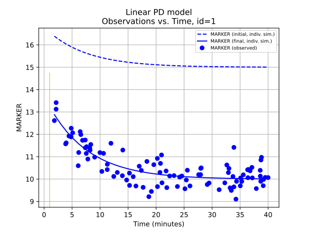
The concentration in the central compartment has a linear effect on the marker response, which is added to a baseline m[BL].

Linear PD models are rarely used because a linear response implies that the bio marker response will be proportional to the drug concentration. This is unlikely to be true in humans because other factors will limit a body’s response to a drug.

Circadian Models

A circadian rhythm is a roughly 24-hour cycle that affects physiological responses in the body. For example, the absorption and metabolisation of a drug can also be faster when taken in the morning compared to the night. Temporal cycles may affect the pharmacokinetics or pharmacodynamics of a drug and so must be taken into account by a model.

Sine Model

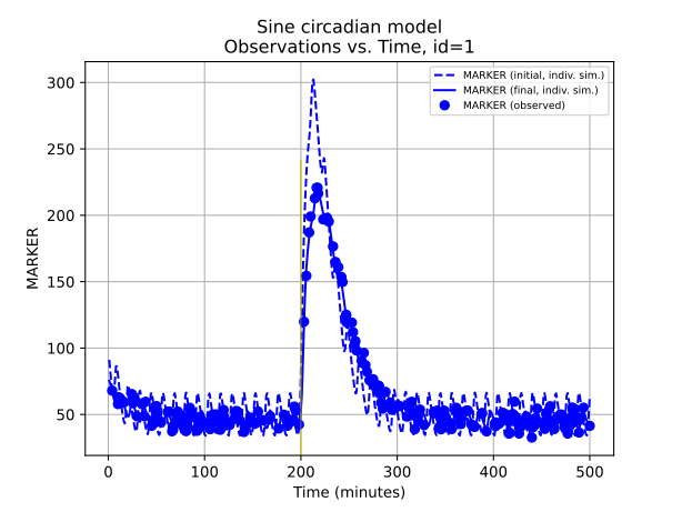
Sine circadian model is a similar example, but this time the sine function is used to replicate the circadian rhythm. The circadian rhythm has been changed to a half-daily rhythm by substituting 12 for 24 in the MODEL_PARAMS section:

MODEL_PARAMS: |
    m[AMP] = f[AMP]
    m[INT] = f[INT]
    m[KOUT] = f[KOUT]
    m[KIN] = c[BASE]*m[KOUT]
    m[ANOISE] = f[ANOISE]

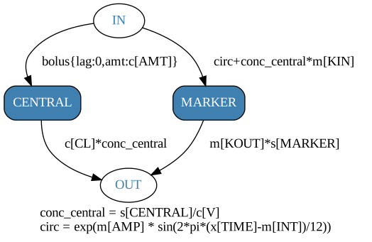
The PD model has also been changed so that the concentration in the central compartment now affects the production of the biomarker and the elimination rate of the biomarker is dependent on the amount of biomarker:

DERIVATIVES: |
    conc_central = s[CENTRAL]/c[V]
    circ = exp(m[AMP] * sin(2*pi*(x[TIME]-m[INT])/12))
    d[CENTRAL] = @bolus{lag:0, amt:c[AMT]} - c[CL]*conc_central  # PK
    d[MARKER] =  m[KIN]*conc_central + circ - m[KOUT]*s[MARKER]  # PD

The compartment diagram is:

Again the PoPy fit script gives good estimates of the ground truth values used to generate the data.

Name	Initial	Fitted	True	Abs. Error	Prop. Error
f[AMP]	3	2…	2	1.79e-03	0.09%
f[INT]	16	7.87	8	1.29e-01	1.61%
f[KOUT]	0.1	0.05…	0.05	1.56e-05	0.03%
f[ANOISE]	5	3.08	3	7.59e-02	2.53%

Emax Models

The response of the human body to a drug is unlikely follow a linear pattern. At low drug concentrations, effects may not occur and/or may be hard to measure. At higher concentrations the effect usually saturates. This is because many of the chemical reactions that occur in the body and are targeted by drugs depend on enzymes.

The effects of drugs often follow a sigmoidal (or S-shaped) curve and an emax model can produce this effect. The emax model is based on the equation

where

and the steepness of the curve is determined by the hill coefficient (), with larger amounts having steeper curves:

Simple Emax Model

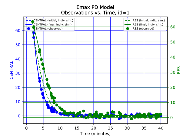
Emax PD Model is a simple emax model. The two compartment PK model is based on previous estimates of K, K12 and K21. The response compartment is based on the amount of drug in the central compartment:

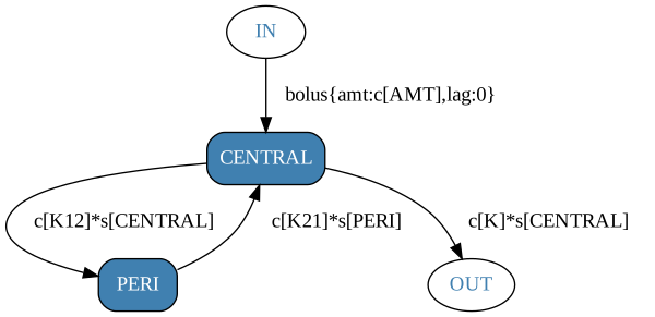
Note that there is no flow out of the response compartment in this model and so the amount in the repsonse compartment grows with each time step.

More Complex Emax Model

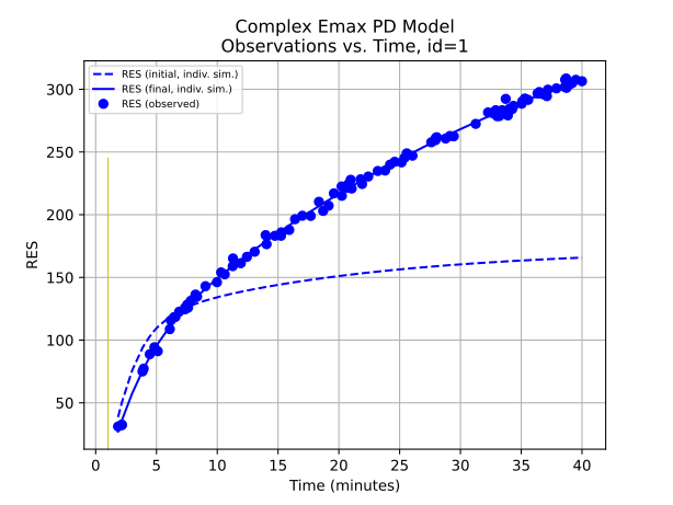
Complex Emax PD Model is a more complex version of Emax PD Model. This model uses the concentration in the central compartment, rather than the amount to influence the response compartment. Concentration is often used instead of amounts because it is the concentration of a drug in the plasma that is measured in clinical trials. This model also has a gamma () parameter to incorporate the steepness of the slope:

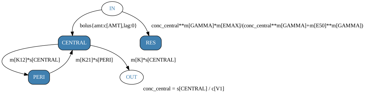
Again, the response accumulates in the response compartment.

Non-Compartmental Response Emax Model

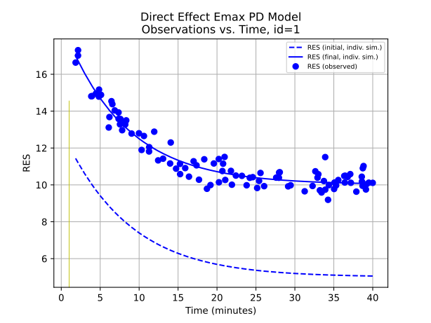
Direct Effect Emax PD Model has a one compartment PK model, but the response variable is outside of the DERIVATIVES block:

DERIVATIVES: |
    d[CENTRAL] = @bolus{amt:c[AMT], lag:0} - m[K]*s[CENTRAL]

and is instead in the PREDICTIONS block:

PREDICTIONS: |
    clabel[TIME] = "Time (minutes)"
    plabel[RES] = 'Response'
    conc = s[CENTRAL]/c[V]
    p[RES] = m[EBASE] + (m[EMAX]*conc)/(m[E50]+conc)
    var =  m[ANOISE]**2
    c[RES] ~ norm(p[RES], var)

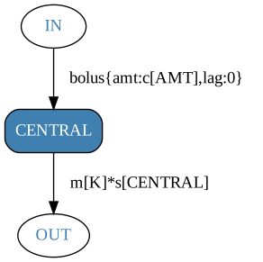
This means the response changes with the concentration in the central compartment and does not accumulate over time. The greater the concentration of drug in the plasma, the greater the response will be.

Biomarker Emax Model

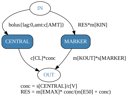
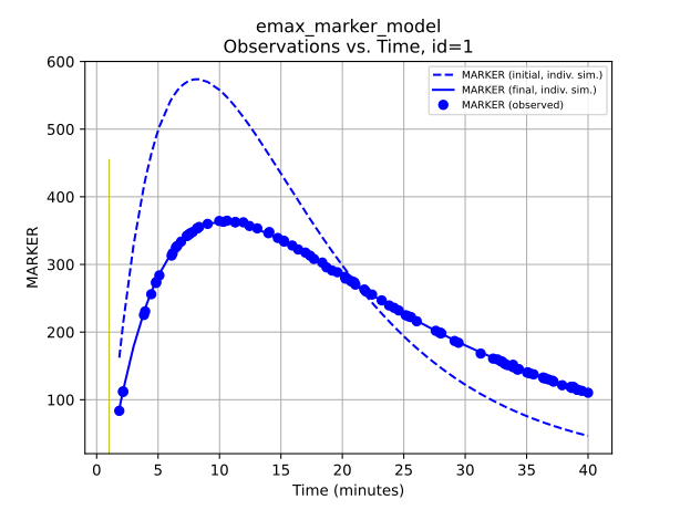
emax_marker_model is an example of a biomarker model. The one compartment PK model estimates the changes in drug concentration in the plasma. This causes a response, which affects the production of a biomarker. The amount of the biomarker being produced increases with increasing drug concentrations:

DERIVATIVES: |
    conc = s[CENTRAL]/c[V]
    d[CENTRAL] = @bolus{lag:0, amt:c[AMT]} - c[CL]*conc
    RES = m[EMAX]* conc/(m[E50] + conc)
    d[MARKER] = m[KIN]*RES - m[KOUT]*s[MARKER]

Other Stuff

• binary response models

• categorical response models

• ordered categorical modelling

• time to event/survival models

• count data

PD Parameter Fitting

In practice PKPD models can be fitted simultaneously or separately (see Separate Vs Simultaneous Fitting).

In the simultaneous case, the model is fitted to PK and PD data at the same time and the m[X] individual PK + PD parameters. deduced at the same time.

In the separate case the PK model is fitted and the PK model parameters for each individuals recorded. The data is then merged with original data set and the PK parameters appear as c[X] variables when fitting the PD model.

In this case study the PD models are demonstrated as the second step in a separate PKPD fit. Therefore PK parameters are assumed to be known (from a prior model fit) and therefore appear as c[X] variables. The PD parameters are m[X] variables, to be deduced by the model.