fit Inputs

As in the gen script, a METHOD_OPTIONS block contains a py_module entry that defines the action to take (fit in this case).

A new FILE_PATHS section includes an input_data_file entry that points to the data file (my_pkpd_model_gen.pyml_output/generated_data/cx_obs_params.csv) that defines the study and the individuals taking part in it.

FILE_PATHS:
    input_data_file: builtin_tut_example_gen.pyml_output/generated_data/cx_obs_params.csv
    output_file_ext: ['svg', 'pdf']

Because the properties of the population and study are entirely contained in the input data, a fit script need only consider what fixed effects and random effects to estimate, so the parent tut script’s FIT_EFFECTS that is copied to the fit script’s EFFECTS block does not include covariates (c[X]) or times (t[X]):

EFFECTS:
    POP: |
        f[KA] ~ P1.0
        f[CL] ~ P1.0
        f[V1] ~ P20
        f[Q] ~ P0.5
        f[V2] ~ P100
        f[KA_isv,CL_isv,V1_isv,Q_isv,V2_isv] ~ spd_matrix() [
            [0.05],
            [0.01, 0.05],
            [0.01, 0.01, 0.05],
            [0.01, 0.01, 0.01, 0.05],
            [0.01, 0.01, 0.01, 0.01, 0.05],
        ]
        f[PNOISE] ~ P0.1
    ID: |
        r[KA, CL, V1, Q, V2] ~ mnorm([0,0,0,0,0], f[KA_isv,CL_isv,V1_isv,Q_isv,V2_isv])

Furthermore, because fixed effects are unknown but allowed to vary they are given a distribution of values (usually to limit their range) and an initial value to begin the estimation process:

f[X] ~ <distribution> <initial value>

For example,

f[X] ~ unif(0.0, +inf) 1.0

defines a uniformly distributed variable that must take a value in the range (0, +infinity) - i.e. a positive value - and that has an initial value of 1.0. Because this range is a common one in PK/PD modelling, PoPy provides a convenient shortcut, ~ P:

f[X] ~ P 1.0

where the ‘P’ is short for ‘positive’.

Random effects definitions are identical to those in the gen script.

In total there are 271 parameters to estimate:

• six univariate parameters

• one symmetric covariance matrix with 15 degrees of freedom

• five random effects for each of the 50 individuals in the population

MODEL_PARAMS, DERIVATIVES and PREDICTIONS define the mathematical model as before, and the ODE_SOLVER section sets the parameters of the solver that integrates derivatives into amounts.

OUTPUT_SCRIPTS defines the subscripts we want to run after completing the model fitting, which in this case are sim, msim and fitsum. As with gen, sim simulates smooth curves at dense time points for the model with estimated (rather than true) values of the parameters, and fitsum creates a HTML report of the fitting process.

msim is a different subscript that, given population fixed effects, will generate many new populations whose statistics can be used to evaluate the goodness of fit via a Visual Predictive Check (VPC).

The other section - also new to the fit script - is the FIT_METHODS section that defines the fitting method (e.g. FOCE, JOE or ND) and its parameters (e.g. tolerances or number of iterations). These parameters control how well and how quickly a fitting algorithm will converge on a final estimate and will be discussed in greater depth later in this book.

FIT_METHODS: [ND: {max_n_main_iterations: 30}]

fit Outputs

Running this fit script (either manually or as part of this tut tutorial), will attempt to minimize iteratively an error function (known as the Objective Function, OBJV) over a number of steps such that the model parameters generate a better prediction of the data at every step. The Objective Function is defined in such a way that it is minimized when the likelihood (the probability of the data given the model) is maximized, and when OBJV stops decreasing the fit is said to have converged (Table 3).

Because the data to which we are fitting with our model was created by simulating observations with the same model, we should expect a good model fit to the data. (Some differences in estimated parameter values should, however, be expected because the observations are noisy and imperfect [Sheiner1980].)

When OBJV has converged to a locally minimal value (a “local minimum”) then the corresponding values of the fixed effects and random effects are returned as the “best” estimates of those variables:

f[KA] = 0.2148
f[CL] = 1.7896
f[V1] = 55.4580
f[Q] = 1.0564
f[V2] = 486.5705
f[KA_isv,CL_isv,V1_isv,Q_isv,V2_isv] = [
    [ 0.1393, -0.0553, 0.0414, -0.0256, 0.1217 ],
    [ -0.0553, 0.0808, -0.0070, -0.0061, -0.1784 ],
    [ 0.0414, -0.0070, 0.1098, -0.0827, 0.2139 ],
    [ -0.0256, -0.0061, -0.0827, 0.3173, -0.3239 ],
    [ 0.1217, -0.1784, 0.2139, -0.3239, 0.9443 ],
]
f[PNOISE] = 0.1415

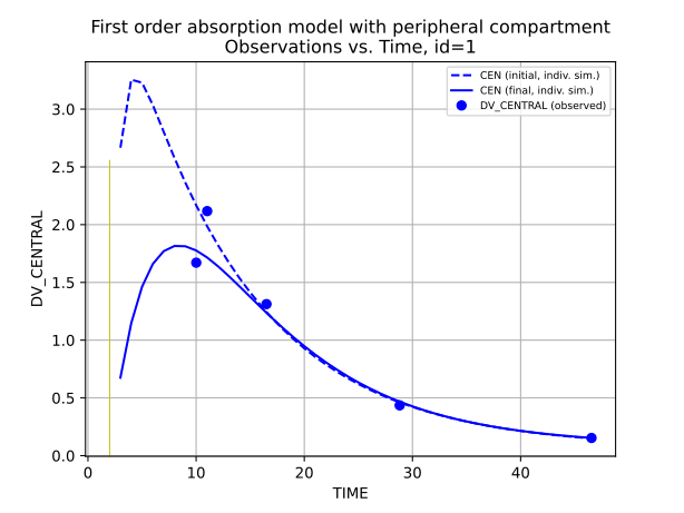
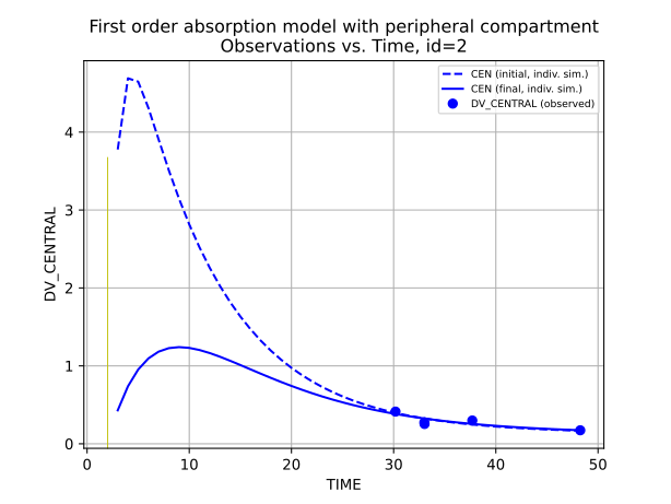
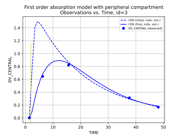
After running fit followed by sim followed by grph we can see a smooth predicted time series of drug concentration for every individual, overlaid with the input observations (Table 4)

Table 4 Model predictions vs original data points for first three individuals

where a dashed blue line represents the noiseless model predictions given the initial f[X] parameters and sampled r[X] values for each individual, a solid blue line represents the predicted curve for the final values, and solid blue dots represent the simulated, noisy observations (c[DV_CENTRAL] in synthetic_data.csv).

These graphs show that PoPy has adjusted the f[X] and r[X] parameters such that the PK curves more closely match the input data and therefore maximise the likelihood of the data being generated from this model.