- Language: en
- Documentation version: 1.3.1
The gen Subscript
The purpose of the Gen Script is to create a synthetic set of data for a population of individuals with properties defined by the user.
To do so, it primarily needs to know about:
the individuals in the population
the specifications of the study or trial (e.g. times of dose and observation)
the mathematical model of the PK/PD
gen Inputs
The properties of the population and study are defined in the
EFFECTS section of the gen script:
EFFECTS:
    POP: |
        c[AMT] = 100.0
        f[KA] = 0.2
        f[CL] = 2.0
        f[V1] = 50
        f[Q] = 1.0
        f[V2] = 80
        f[KA_isv,CL_isv,V1_isv,Q_isv,V2_isv] = [
            [0.1],
            [0.01, 0.03],
            [0.01, -0.01, 0.09],
            [0.01, 0.02, 0.01, 0.07],
            [0.01, 0.02, 0.01, 0.01, 0.05],
        ]
        f[PNOISE] = 0.15
    ID: |
        c[ID] = sequential(50)
        t[DOSE] = 2.0
        t[OBS] ~ unif(1.0, 50.0; 5)
        # t[OBS] = range(1.0, 50.0; 5)
        r[KA, CL, V1, Q, V2] ~ mnorm([0,0,0,0,0], f[KA_isv,CL_isv,V1_isv,Q_isv,V2_isv])
which is a carbon copy of the
GEN_EFFECTS section of the parent tut script.
Very briefly, this EFFECTS section defines a population of 50 individuals,
numbered sequentially from 1 to 50,
c[ID] = sequential(50)
numerous fixed effects with constant values (as indicated by the use of the “=” assignment operator),
f[KA] = 0.2
f[CL] = 2.0
...
and random effects that are sampled (as indicated by the use of the “~” distribution operator) for each individual from a zero-mean, multi-variate normal distribution whose symmetric positive definite covariance matrix (specified completely by its lower triangular elements) is defined by one of the population-level fixed effects,
f[KA_isv,CL_isv,V1_isv,Q_isv,V2_isv] = [
    [0.1],
    [0.01, 0.03],
    [0.01, -0.01, 0.09],
    [0.01, 0.02, 0.01, 0.07],
    [0.01, 0.02, 0.01, 0.01, 0.05],
]
...
r[KA, CL, V1, Q, V2] ~ mnorm([0,0,0,0,0], f[KA_isv,CL_isv,V1_isv,Q_isv,V2_isv])
Regarding the study properties, it defines a dose of 100 units of drug,
administered at time t = 2.0,
c[AMT] = 100.0
...
t[DOSE] = 2.0
and five observations at time points uniformly distributed in the period [1.0, 50.0]:
t[OBS] ~ unif(1.0, 50.0; 5)
with a hierarchical structure that includes between-subject variability but no between-occasion variability,
POP: |
    # population-level parameters
ID: |
    # individual-level parameters
In PoPy, POP is the root of the hierarchy which, in this example,
creates an ID branch for every unique value of c[ID] (50 branches in
this case).
Covariates and random effects defined at the ID level
will be resampled for every ID branch.
In contrast, population-level fixed effects are
treated as if defined at the POP level, wherever they
happen to be defined. (This allows you to define population covariances
immediately before random effect distributions that depend upon them.)
Deeper levels of the hierarchy (e.g. between-occasion variability) can be
created by adding more entries to the tree structure, e.g. below ID.
Time definitions must be at the lowest level of the hierarchy because
they implicitly define the leaves of the tree structure (one leaf node
per row).
The mathematical model to be simulated is defined by the MODEL_PARAMS,
STATES, DERIVATIVES and PREDICTIONS sections,
all of which are carbon copies of the corresponding sections in the tut
script.
In this built-in example, the model is a two compartment model
with absorption and bolus dosing (Fig. 3:)
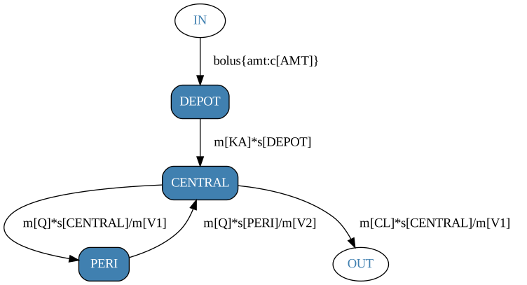
Fig. 3 Two compartment model with depot dosing for Tut Script.
but the exact details of the model are not important here.
One distinction is, however, worth noting: the PREDICTIONS section
defines the probability distribution of the observation (c[DV_CENTRAL])
var = m[ANOISE]**2 + m[PNOISE]**2 * p[DV_CENTRAL]**2
c[DV_CENTRAL] ~ norm(p[DV_CENTRAL], var)
which, for a gen script, is sampled at every observation time point
in order to simulate noisy observations.
The remaining sections of note at this point include:
METHOD_OPTIONS: derived from thetutscript but withpy_moduleset togenso that PoPy knows which action to applyODE_SOLVER: a carbon copy of the same section in thetutscript, setting the parameters of the ODE solver that will simulate the compartment modelOUTPUT_SCRIPTS: the subscripts ofgento be run, which are populated with default values
The ability to generate synthetic data from a model is especially useful if you wish to demonstrate a model, but do not have access to a real data set. Real data is expensive to obtain and even if it exists may have issues regarding completeness, accuracy or confidentiality. The other disadvantage of real data is that we never know the true underlying model.
gen Outputs
The main gen output is a machine-readable tabular file, stored at
<tutorial script output folder>\
    my_pkpd_model_gen.pyml_output\
        synthetic_data.csv
that contains both assigned (or sampled) covariates and sampled observations.
whose first few ten rows are shown in (Table 1).
TIME |
ID |
TYPE |
AMT |
DV_CENTRAL |
DV_CENTRAL_FLAG |
orig_data_row |
|---|---|---|---|---|---|---|
2 |
1 |
dose |
100 |
0.00152359650281 |
0 |
0 |
10.0120217722 |
1 |
obs |
100 |
1.67075294237 |
1 |
1 |
11.0234536491 |
1 |
obs |
100 |
2.11707619384 |
1 |
2 |
16.5024021745 |
1 |
obs |
100 |
1.31206960996 |
1 |
3 |
28.818526425 |
1 |
obs |
100 |
0.435327698431 |
1 |
4 |
46.551188548 |
1 |
obs |
100 |
0.153098540708 |
1 |
5 |
2 |
2 |
dose |
100 |
0.000377833830139 |
0 |
0 |
30.181690446 |
2 |
obs |
100 |
0.412763665129 |
1 |
1 |
33.0056777467 |
2 |
obs |
100 |
0.274939718447 |
1 |
2 |
… |
… |
… |
… |
… |
… |
… |
This data file, combining covariates and observations, is effectively what you would input to a parameter estimation program to fit a model to data.
The data file starts with a header row that labels the covariates so that they can be referenced by name in downstream processes. In this example, the column/covariate labels are:
TYPE: whether the row is a dose, an observation or a simulation
ID: the identifier for a given individual
TIME: the time stamp of the row event
AMT: the amount of drug administered if the row is of dose TYPE
DV_CENTRAL: the simulated observation
DV_CENTRAL_FLAG: whether the observation should be classed as a measurement in parameter estimation
orig_data_row: the data row number within an individual subject
Intermediate outputs of gen are saved to files in
<tutorial script output folder>\
    my_pkpd_model_gen.pyml_output\
        generated_data\
and include:
assigned (or sampled) fixed effects, stored in a machine-readable
fx_params.csvtabular filesampled random effects, stored in a machine-readable
rx_params.csvtabular file
These outputs are generated in two stages: sampling and simulation.
The sampling stage proceeds in four steps:
First, population-level fixed effects f[X] variables defined in the EFFECTS section
are assigned or sampled. (In this case the f[X] are all assigned constants.)
Second, a hierarchical tree structure of covariates is created by assigning
or sampling values according to their position in the EFFECTS section.
In this example, we sample 50 unique individuals who share a common AMT
covariate at the POP level.
(The c[TIME] and c[TYPE] fields are created by PoPy automatically.)
Third, we sample (never assign) random effects following the same hierarchy, applying dependencies on the (known) fixed effects.
Fourth, we assign or sample dose and observation times at every leaf of the tree structure. In this example, we assign one dose time and sample five observation times for each of the 50 individuals, giving a dataset of 300 rows in total.
The simulation step then uses these sampled values to compute PK/PD model
parameters, initial compartment amounts, the compartment amount at every
sampled time point, and a simulated noisy observation at every time point according to
the MODEL_PARAMS, STATES, DERIVATIVES and PREDICTIONS sections,
respectively.
These simulated observations are then combined with the sampled values
and saved to synthetic_data.csv.
Subscripts of gen can be used to plot the simulated observations (grph);
simulate smooth, noiseless curves of the time series (sim); and summarize the
generated data in an HTML report (gensum).
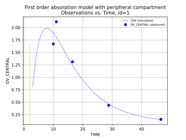
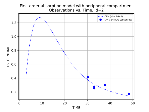
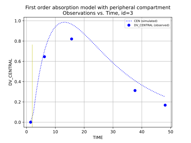
We can see (in Table 2)
the first three plots created by
gen followed by sim followed by grph.
Here, a dotted blue line represents the noiseless model predictions
given the f[X] parameters and sampled r[X] values for each individual, and
solid blue dots represent the simulated, noisy observations
(c[DV_CENTRAL] in synthetic_data.csv).
|
|
|